
Almost nothing. A failed assumption check does not invalidate your dissertation and rarely forces you to abandon your planned test. Each assumption has a specific remedy — a robust correction, a transformation, a bootstrap, or a non-parametric alternative — and the choice depends on which assumption failed, how badly, and how large your sample is. Reporting the failure and your response is what earns marks.
Most students meet this at the worst possible moment: analysis week, output on screen, a significance value where they wanted a non-significant one. The panic move is to swap to a non-parametric test and hope. That is sometimes right and often the weakest of the available options. Here is what each failure actually means and what to do about it.
This guide assumes you have already chosen your test; if you have not, start with our decision guide to choosing the right statistical test and come back here when a check fails.
Why does a significant normality test not automatically mean trouble?
Because significance tests of normality answer a question about your sample size as much as about your data. The Shapiro-Wilk test asks whether your data depart detectably from a normal distribution. With a small sample it lacks the power to detect real departures; with a large one it flags departures so slight they have no practical consequence. The same data can pass at n = 25 and fail at n = 300.
So a significant Shapiro-Wilk is a prompt to look, not a verdict. Open a histogram and a Q-Q plot and ask a different question: is this a mild skew, or is it bimodal, heavily tailed, or dominated by a floor or ceiling effect? Mild skew in a reasonable sample is usually survivable. A bimodal distribution is telling you something substantive about your sample that no test switch will fix.
What exactly has to be normal?
Not what most students check. Three clarifications that resolve a great deal of unnecessary alarm:
- For a t-test or ANOVA, the assumption concerns the distribution of scores within each group, not the pooled outcome variable. Running Shapiro-Wilk on everyone together, when your two groups genuinely differ, can produce a failure caused by the effect you are trying to detect.
- For regression, the assumption concerns the residuals, not the predictors and not the outcome. Testing your variables for normality before a regression is checking something the model never assumed.
- Strictly, the assumption is about the sampling distribution of the statistic. As sample size grows, that distribution tends towards normality even when the underlying data are not normal, which is why moderate departures matter less as n increases.
Check the right thing first. A surprising share of assumption crises dissolve at this step.
What are the options when normality genuinely fails?
Four, roughly in order of preference:
- Proceed and report. With a decent sample size and a modest departure, run the parametric test, state that the assumption was violated, describe the departure, and explain why you proceeded. This is a defensible, common decision — provided you say so rather than hiding it.
- Bootstrap. Bootstrapping resamples your data to build an empirical sampling distribution and produces confidence intervals that do not rest on the normality assumption. SPSS offers it as a button in many dialogs. It keeps your original test and its interpretation, which is why it beats switching tests.
- Transform the variable. A log transformation for positive skew, a square root for count-like data. The cost is interpretive: your results are now about log units, and every mean, coefficient and confidence interval has to be discussed on that scale or back-transformed carefully. Do not transform unless you are willing to write about the transformed variable.
- Switch to a non-parametric test. Robust to distribution shape, but it tests a different hypothesis — broadly about ranks rather than means — and generally has less power when the parametric assumptions would have held.
Which non-parametric test replaces which parametric one?
| Parametric test | Non-parametric alternative | What it compares |
|---|---|---|
| Independent-samples t-test | Mann-Whitney U | Two independent groups |
| Paired-samples t-test | Wilcoxon signed-rank | Two related measurements |
| One-way ANOVA | Kruskal-Wallis H | Three or more independent groups |
| Repeated-measures ANOVA | Friedman | Three or more related measurements |
| Pearson’s r | Spearman’s rho | Monotonic association between two variables |
Two things to remember when you use one. Report the appropriate descriptive statistics — medians and interquartile ranges rather than means and standard deviations — because reporting means alongside a rank-based test is inconsistent. And note that these tests are not assumption-free: several carry a similar-distribution-shape assumption of their own if you want to interpret them as comparing medians.
What if Levene’s test says the variances are unequal?
This is the easiest failure to handle, because the fix is already in your output. For a t-test, read the “Equal variances not assumed” row — the Welch correction — and report its decimal degrees of freedom, exactly as set out in our walkthrough of the independent-samples t-test in SPSS. For a one-way ANOVA, request Welch’s F in the Options dialog and report that instead of the standard F, then use Games-Howell rather than Tukey for your post-hoc comparisons.
There is no need to switch to a non-parametric test for unequal variances alone. Doing so is over-correction, and it costs you the ability to talk about means.
What if Mauchly’s test of sphericity is significant?
Sphericity applies to repeated-measures designs with three or more conditions, and it concerns whether the variances of the differences between conditions are equal. When Mauchly’s test is significant, you do not change test — you apply a correction to the degrees of freedom and read the corrected row that SPSS has already produced.
The Greenhouse-Geisser correction is the conservative default and the safe choice for a dissertation; Huynh-Feldt is less conservative and preferred by some when the violation is mild. Report which correction you used and give the adjusted, non-integer degrees of freedom. Never report Mauchly’s test and then read the uncorrected row anyway, which is a startlingly common error.
What if my regression has multicollinearity?
Multicollinearity means two or more predictors carry largely the same information, which destabilises the individual coefficients even when the model as a whole fits well. The diagnostic is the variance inflation factor: commonly used thresholds treat a VIF above 10 as a serious problem and above 5 as worth investigating, with tolerance (its reciprocal) read in the opposite direction.
The remedies are conceptual rather than statistical. Drop one of the offending predictors, keeping the one your theory says matters. Combine them into a single composite or scale score if they are measuring the same construct — which is itself a question about internal consistency. Or centre the variables where the collinearity comes from an interaction term you constructed. What you cannot do is ignore it and interpret the individual coefficients as though each predictor’s contribution were cleanly separated.

What about the other regression assumptions?
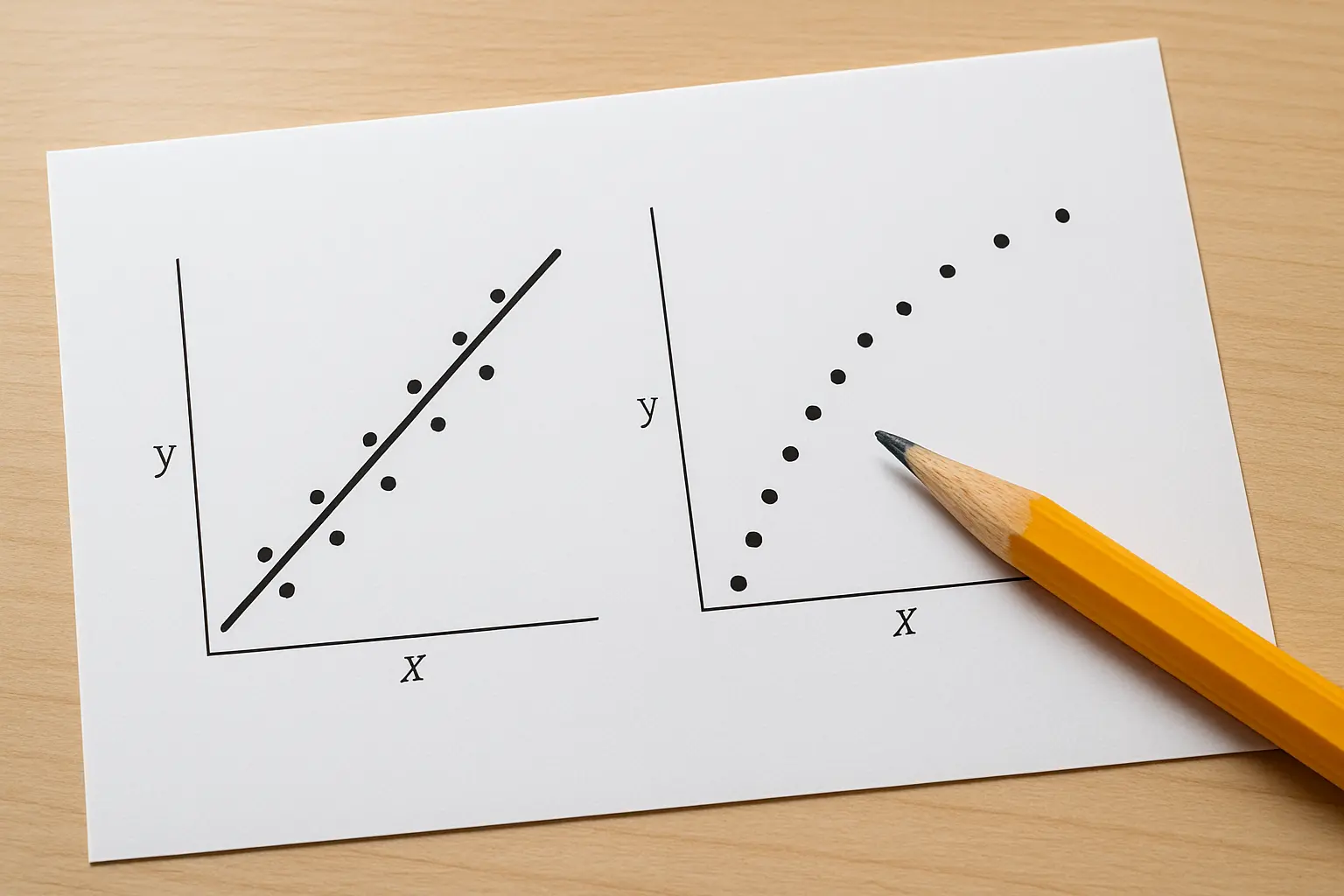
Linearity. Plot the residuals against the predicted values. A curved pattern means the relationship is not linear; add a quadratic term or transform the predictor rather than reporting a linear model that misdescribes your data.
Homoscedasticity. The same plot. A funnel shape — residuals spreading out as predicted values increase — means the error variance is not constant. Robust standard errors or bootstrapped confidence intervals are the usual answers.
Independence of residuals. The Durbin-Watson statistic ranges from 0 to 4, with values near 2 indicating no autocorrelation and roughly 1.5 to 2.5 conventionally treated as acceptable. Genuine autocorrelation usually signals that your design has structure — repeated measurements, participants clustered in classes or wards — that a simple regression is not modelling.
What should you never do?
Four things, all of which are visible to a marker who reads carefully.
Do not delete cases because they are inconvenient. Genuine outliers may be excluded with a stated, pre-specified rule; cases removed until the assumption passes are data manipulation, and reporting both the full and reduced analyses is the honest route when you are unsure.
Do not run every test and report only the one that gave you a significant result. If you ran both a t-test and a Mann-Whitney, say so and say why you preferred one.
Do not report an assumption check and then behave as though it passed. The corrected row exists; use it.
And do not silently omit the checks. An examiner who cannot see that you tested the assumptions will assume you did not.
How do you write this up?
Assumption checks belong in your results chapter, briefly, before the test they precede — not in a separate appendix nobody reads. A single paragraph does it:
“Normality was assessed using Shapiro-Wilk tests and visual inspection of Q-Q plots. Scores in the control group departed significantly from normality, W(29) = 0.91, p = .017, although inspection indicated only mild positive skew. Given the sample size and the modest departure, the parametric test was retained and bootstrapped 95% confidence intervals (1,000 resamples) are reported alongside it.”
That paragraph reports the check, describes the violation, names the decision and justifies it. It takes sixty words and it is the difference between a marker reading a considered analysis and reading an unexamined one. The wider structure it sits in — where analysis decisions are stated and defended — is set out in our guide to writing a methodology chapter, and if your sample was small enough that power is part of the story, that reasoning belongs in the same discussion as your sample size justification.
When the analysis is settled and the chapters are what stand between you and submission, Tesify can structure and draft your dissertation around your own results — every word still written by you.
Frequently asked questions
My data are not normally distributed. Can I still use a t-test?
Often yes. Check whether the departure is mild, whether your sample is reasonably large, and whether you checked normality within groups rather than overall. Then either proceed with a stated justification, bootstrap the confidence intervals, or switch to Mann-Whitney — and report whichever you chose.
Should I use Shapiro-Wilk or Kolmogorov-Smirnov?
Shapiro-Wilk is generally the more sensitive of the two at the sample sizes typical of a dissertation, and SPSS reports both. Whichever you use, read the plots as well; the test alone is too dependent on sample size to be trusted on its own.
Is it cheating to transform my data?
No, provided you report it and interpret the results on the transformed scale or back-transform carefully. Transformation becomes a problem only when it is undisclosed, or when a student transforms repeatedly until something turns significant.
Can I remove outliers to fix normality?
Only with a pre-specified, stated rule, and you should report the analysis with and without them. Removing cases until an assumption passes is not an assumption check; it is a way of choosing your result.
Do non-parametric tests have assumptions too?
Yes. Independence of observations still applies, and interpreting Mann-Whitney or Kruskal-Wallis as a comparison of medians assumes similarly shaped distributions across groups. They are more robust, not assumption-free.
What do I do if there is no non-parametric equivalent for my design?
This is common in factorial and mixed designs. Bootstrapping, robust standard errors or a generalised linear model with an appropriate distribution are the usual routes, and your supervisor is the right person to ask before you commit.
Does a big sample mean I can ignore normality?
It means moderate departures matter less, because the sampling distribution of the mean tends towards normality as n grows. It does not license ignoring a bimodal distribution or severe outliers, which usually indicate something real about your sample.
Levene’s test is significant. Do I need a non-parametric test?
No. Use the Welch correction — the “equal variances not assumed” row for a t-test, Welch’s F for an ANOVA with Games-Howell post-hoc tests. Switching to a rank-based test for unequal variances alone gives up more than it gains.
How do I report Greenhouse-Geisser corrected results?
State that Mauchly’s test indicated a violation of sphericity, give its value, then report the F test with the corrected non-integer degrees of freedom and name the correction used. The corrected row is already in your SPSS output.
Will I lose marks for a violated assumption?
Very rarely for the violation itself, and reliably for concealing it. Markers assess whether you noticed, whether you understood the consequence and whether your response was sensible. A well-handled violation is evidence of competence, not a flaw in the project.