
Tag: quantitative dissertation

  • How to Run an Independent-Samples T-Test in SPSS and Report It Properly (2026)

    How to Run an Independent-Samples T-Test in SPSS and Report It Properly (2026)

    You have your data, your deadline is close, and you need one number out of SPSS and one sentence into your results chapter. This guide takes you from a spreadsheet to that sentence, with the expected output of each step stated so you can tell you have done it correctly.

    An independent-samples t-test compares the mean of one continuous outcome between two separate groups of people — men and women, intervention and control, first years and final years. If the same people were measured twice, you need the paired-samples test instead, and the procedure differs. If the analysis is under control and the writing is not, you can draft your results chapter in Tesify.

    Step 1: Confirm the t-test is the right test

    Three conditions. Your outcome variable is continuous — a score, a time, a measurement — not a category and not a rank. Your predictor is a single categorical variable with exactly two levels. And each participant appears in one group only.

    Three levels rather than two means a one-way ANOVA. The same people measured before and after means a paired-samples test. A categorical outcome means a chi-square. If any of that is uncertain, work through our decision guide to choosing the right statistical test before you touch the software, because running the wrong test correctly is still the wrong test.

    Expected output: a written sentence naming your outcome variable, your grouping variable and its two levels.

    Step 2: Get the data into the right shape

    This is where most of the lost time goes, and it is entirely mechanical. SPSS needs long format: one row per participant, one column for the grouping variable and one column for the outcome. Students who arrive with the two groups in two side-by-side columns — a perfectly natural spreadsheet layout — cannot run the test until they restructure.

    1. Enter or import your data so each participant occupies a single row.
    2. Create the grouping variable as a numeric variable coded 1 and 2, and set its Values in Variable View so 1 = Control and 2 = Intervention. Labels are what make your output readable months later.
    3. Set the outcome variable’s Measure to Scale.
    4. Check for missing values and decide, deliberately, how you are handling them — then say so in your methods.
    5. Reverse-score any negatively worded questionnaire items before computing a total score. If your outcome is a scale total, this is also the point at which you compute reliability; see our guide to an acceptable Cronbach’s alpha.

    Expected output: a dataset with labelled variables, one row per participant, and a total score computed if you need one.

    A dataset laid out with a grouping variable and an outcome variable ready for analysis
    Long format: one row per participant, a coded grouping column, a scale outcome column. Everything downstream depends on this.

    Step 3: Run the test

    Go to Analyze → Compare Means → Independent-Samples T Test. In recent SPSS versions that submenu is labelled Compare Means and Proportions; the dialog is the same.

    1. Move your outcome variable into Test Variable(s).
    2. Move your grouping variable into Grouping Variable. It will show two question marks.
    3. Click Define Groups and enter your two codes — 1 and 2 — then Continue. Skipping this is the single most common reason the OK button stays greyed out.
    4. If your version offers an Estimate effect sizes checkbox in the dialog, tick it now; it saves calculating Cohen’s d by hand later.
    5. Click OK.

    Expected output: two tables in the output viewer — Group Statistics, and Independent Samples Test.

    Step 4: Read the Group Statistics table

    This table gives you N, mean, standard deviation and standard error for each group. Read it before you look at anything else, for two reasons: it tells you whether your groups are the size you think they are, and it tells you the direction of any difference. A significant p value means nothing to a reader who does not know which group scored higher.

    Write the four numbers down now — both means and both standard deviations — because they go into your reporting sentence and you will otherwise scroll back for them.

    Step 5: Read the Independent Samples Test table — and pick the right row

    This table has two rows for your variable, and choosing between them is the step students get wrong most often.

    The first columns show Levene’s Test for Equality of Variances, which asks whether the two groups’ spread of scores is similar. Read its significance value:

    • Levene’s p is above .05 — variances can be treated as equal. Read the top row, “Equal variances assumed”.
    • Levene’s p is .05 or below — the equal-variance assumption has failed. Read the bottom row, “Equal variances not assumed”. This is the Welch correction; it adjusts the degrees of freedom, which is why they come out as a decimal such as 41.283.

    Two things worth knowing. Levene’s own p value is not a finding and does not belong in your results prose — it selects your row, nothing more. And a failed Levene’s test is not a disaster: SPSS has already handled it, and you simply report the Welch row with its decimal degrees of freedom, noting that you did. Some statisticians argue for reporting the Welch row routinely regardless. Follow what your department teaches, and be consistent.

    From your chosen row, take three numbers: t, df, and the significance value. Take the 95% confidence interval of the difference as well — APA expects it and most students omit it.

    Expected output: t, df, p and the 95% CI, from one row you can justify choosing.

    Step 6: Get the effect size

    A p value tells you whether a difference is unlikely under the null hypothesis; it says nothing about how big the difference is. Cohen’s d says how big, expressed in standard deviations, and markers increasingly expect it.

    If SPSS produced an effect-sizes table, take Cohen’s d from it. If not, d is the difference between the two means divided by the pooled standard deviation. Interpret it with the conventional benchmarks — around 0.2 small, 0.5 medium, 0.8 large — and treat them as rough orientation rather than law, exactly as with the conventions used for sample size and power.

    The pairing that impresses a marker is a modest effect size honestly reported next to a significant p value, with a sentence acknowledging what that combination means.

    Step 7: Write the reporting sentence

    APA style wants the descriptive statistics, the test statistic with its degrees of freedom, an exact p value, and the effect size. Here is a complete worked example you can adapt:

    An independent-samples t-test compared exam anxiety scores between the intervention group (M = 24.10, SD = 5.62, n = 31) and the control group (M = 28.45, SD = 5.91, n = 29). Levene’s test indicated equal variances, F(1, 58) = 0.42, p = .520. The intervention group reported significantly lower anxiety than the control group, t(58) = −2.92, p = .005, 95% CI [−7.33, −1.37], d = 0.75, a medium-to-large effect.

    And the version where Levene’s test failed:

    Because Levene’s test indicated unequal variances, F(1, 58) = 6.11, p = .016, the Welch correction was applied. The difference was significant, t(48.72) = −2.71, p = .009, 95% CI [−7.61, −1.12], d = 0.70.

    Formatting details that cost easy marks: no leading zero before a decimal that cannot exceed one, so p = .005 and not 0.005; report exact p values to two or three decimals, using p < .001 only when the value is smaller than that; italicise the statistical symbols but not the brackets or numerals; and never write p = .000, which SPSS displays as a rounding artefact and which is not a real value.
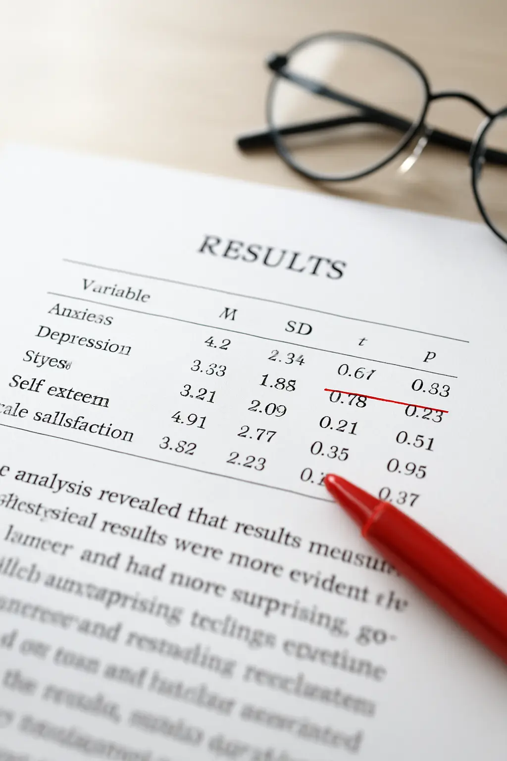
    A dissertation results chapter with a formatted statistics table and reporting sentence
    The table shows the numbers; the sentence says what they mean and in which direction. A results chapter needs both.

    Step 8: Build the table, and say what it means

    For a single t-test a table is optional and the sentence alone is usually cleaner. For several comparisons, build one table with a row per outcome and columns for each group’s M and SD, then t, df, p and d. Never present the raw SPSS output as your table — pasted SPSS screenshots in a results chapter read as unfinished work. Retype the numbers into a properly formatted table with a title above it.

    Then, in the discussion, interpret. A significant result answers your hypothesis; it does not explain itself. What might produce a four-point difference in anxiety, and does it match what your literature review predicted?

    Five errors that cost marks

    1. Reading the wrong Levene’s row. Covered above, and it changes both your df and often your p.
    2. Reporting p = .000. Write p < .001.
    3. Omitting the effect size. Increasingly treated as a requirement rather than a nicety.
    4. Not saying which group was higher. A t value’s sign depends on your group coding, so a reader cannot infer direction from it. State the means.
    5. Treating a non-significant result as a failure. It is a finding. Report it fully, give the effect size and confidence interval, and discuss statistical power rather than apologising.

    What if you do not have SPSS?

    The procedure transfers. jamovi and JASP run the same test through a similar dialog and output the effect size and confidence interval by default; in R it is a single line. Which package suits an undergraduate dissertation, and what your department is likely to support, is covered in our comparison of SPSS, R and jamovi. Whichever you use, name it and its version in your methodology chapter.

    When the numbers are settled and the chapters need writing, Tesify can structure and draft your dissertation around your own results — the analysis and every word remain yours, with the structure and bibliography handled.

    Frequently asked questions

    What is the difference between an independent-samples and a paired-samples t-test?

    Independent samples compares two separate groups of people. Paired samples compares the same people on two occasions, or matched pairs. Using the independent test on repeated measures throws away the pairing and loses statistical power.

    Which row do I read if Levene’s test is significant?

    The bottom row, “Equal variances not assumed”. Its degrees of freedom will be a decimal because the Welch correction adjusts them. Report that row and note in your text that the correction was applied.

    Do I have to report Levene’s test in my results?

    A short clause is good practice because it justifies which row you read. It is not a finding in its own right, so keep it to one clause rather than giving it a paragraph.

    Why is my t value negative?

    Because SPSS subtracts group 2’s mean from group 1’s. The sign reflects your coding, not the importance of the result. Report it as SPSS gives it and make the direction clear by stating both means.

    How do I report a non-significant t-test?

    Exactly as you would a significant one — means, standard deviations, t, df, exact p, confidence interval and effect size — then discuss it. A non-significant result with a wide confidence interval and a small sample is a power problem worth naming in your limitations.

    What sample size do I need for a t-test?

    It depends on the effect size you expect and the power you want. Decide it in advance rather than after collecting data, using the reasoning set out in our sample size guide, and report the justification in your methods.

    Can I run a t-test on Likert data?

    A total score summed across several Likert items is normally treated as continuous and analysed with a t-test. A single Likert item is ordinal, and a Mann-Whitney U test is the safer choice. Departments differ on this, so check what yours teaches.

    What do I do if my data are not normally distributed?

    Do not panic and do not immediately abandon the t-test. Sample size, the shape of the departure and the specific assumption that failed all matter, and there are several routes forward besides switching test.

    Should I report the confidence interval?

    Yes. It tells the reader the range of plausible values for the true difference, which a p value does not, and APA style expects it. SPSS gives it to you in the same row you already read.

    Can I paste the SPSS output straight into my dissertation?

    No. Retype the numbers into a table formatted to your department’s style. Raw output belongs in an appendix if anywhere, and a chapter of pasted screenshots looks like a student who ran out of time.

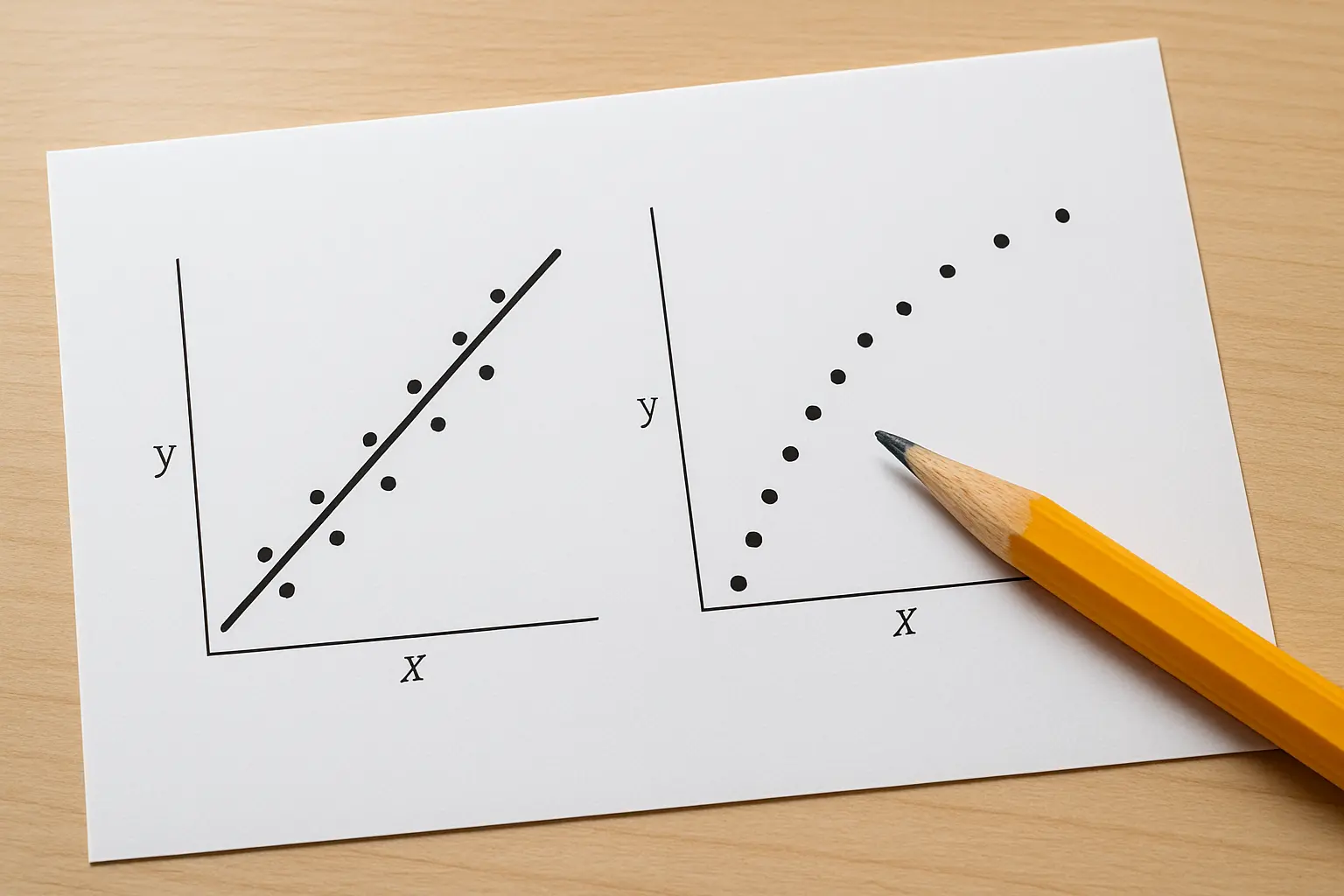
  • What Do You Do When Your Statistical Assumptions Fail? (2026)

    What Do You Do When Your Statistical Assumptions Fail? (2026)

    Almost nothing. A failed assumption check does not invalidate your dissertation and rarely forces you to abandon your planned test. Each assumption has a specific remedy — a robust correction, a transformation, a bootstrap, or a non-parametric alternative — and the choice depends on which assumption failed, how badly, and how large your sample is. Reporting the failure and your response is what earns marks.

    Most students meet this at the worst possible moment: analysis week, output on screen, a significance value where they wanted a non-significant one. The panic move is to swap to a non-parametric test and hope. That is sometimes right and often the weakest of the available options. Here is what each failure actually means and what to do about it.

    This guide assumes you have already chosen your test; if you have not, start with our decision guide to choosing the right statistical test and come back here when a check fails.

    Why does a significant normality test not automatically mean trouble?

    Because significance tests of normality answer a question about your sample size as much as about your data. The Shapiro-Wilk test asks whether your data depart detectably from a normal distribution. With a small sample it lacks the power to detect real departures; with a large one it flags departures so slight they have no practical consequence. The same data can pass at n = 25 and fail at n = 300.

    So a significant Shapiro-Wilk is a prompt to look, not a verdict. Open a histogram and a Q-Q plot and ask a different question: is this a mild skew, or is it bimodal, heavily tailed, or dominated by a floor or ceiling effect? Mild skew in a reasonable sample is usually survivable. A bimodal distribution is telling you something substantive about your sample that no test switch will fix.

    Two diagnostic plots compared, one following the reference line and one departing from it
    A Q-Q plot answers a more useful question than a significance test: not whether the departure is detectable, but whether it is large.

    What exactly has to be normal?

    Not what most students check. Three clarifications that resolve a great deal of unnecessary alarm:

    • For a t-test or ANOVA, the assumption concerns the distribution of scores within each group, not the pooled outcome variable. Running Shapiro-Wilk on everyone together, when your two groups genuinely differ, can produce a failure caused by the effect you are trying to detect.
    • For regression, the assumption concerns the residuals, not the predictors and not the outcome. Testing your variables for normality before a regression is checking something the model never assumed.
    • Strictly, the assumption is about the sampling distribution of the statistic. As sample size grows, that distribution tends towards normality even when the underlying data are not normal, which is why moderate departures matter less as n increases.

    Check the right thing first. A surprising share of assumption crises dissolve at this step.

    What are the options when normality genuinely fails?

    Four, roughly in order of preference:

    1. Proceed and report. With a decent sample size and a modest departure, run the parametric test, state that the assumption was violated, describe the departure, and explain why you proceeded. This is a defensible, common decision — provided you say so rather than hiding it.
    2. Bootstrap. Bootstrapping resamples your data to build an empirical sampling distribution and produces confidence intervals that do not rest on the normality assumption. SPSS offers it as a button in many dialogs. It keeps your original test and its interpretation, which is why it beats switching tests.
    3. Transform the variable. A log transformation for positive skew, a square root for count-like data. The cost is interpretive: your results are now about log units, and every mean, coefficient and confidence interval has to be discussed on that scale or back-transformed carefully. Do not transform unless you are willing to write about the transformed variable.
    4. Switch to a non-parametric test. Robust to distribution shape, but it tests a different hypothesis — broadly about ranks rather than means — and generally has less power when the parametric assumptions would have held.

    Which non-parametric test replaces which parametric one?

    Parametric test Non-parametric alternative What it compares
    Independent-samples t-test Mann-Whitney U Two independent groups
    Paired-samples t-test Wilcoxon signed-rank Two related measurements
    One-way ANOVA Kruskal-Wallis H Three or more independent groups
    Repeated-measures ANOVA Friedman Three or more related measurements
    Pearson’s r Spearman’s rho Monotonic association between two variables

    Two things to remember when you use one. Report the appropriate descriptive statistics — medians and interquartile ranges rather than means and standard deviations — because reporting means alongside a rank-based test is inconsistent. And note that these tests are not assumption-free: several carry a similar-distribution-shape assumption of their own if you want to interpret them as comparing medians.

    What if Levene’s test says the variances are unequal?

    This is the easiest failure to handle, because the fix is already in your output. For a t-test, read the “Equal variances not assumed” row — the Welch correction — and report its decimal degrees of freedom, exactly as set out in our walkthrough of the independent-samples t-test in SPSS. For a one-way ANOVA, request Welch’s F in the Options dialog and report that instead of the standard F, then use Games-Howell rather than Tukey for your post-hoc comparisons.

    There is no need to switch to a non-parametric test for unequal variances alone. Doing so is over-correction, and it costs you the ability to talk about means.

    What if Mauchly’s test of sphericity is significant?

    Sphericity applies to repeated-measures designs with three or more conditions, and it concerns whether the variances of the differences between conditions are equal. When Mauchly’s test is significant, you do not change test — you apply a correction to the degrees of freedom and read the corrected row that SPSS has already produced.

    The Greenhouse-Geisser correction is the conservative default and the safe choice for a dissertation; Huynh-Feldt is less conservative and preferred by some when the violation is mild. Report which correction you used and give the adjusted, non-integer degrees of freedom. Never report Mauchly’s test and then read the uncorrected row anyway, which is a startlingly common error.

    What if my regression has multicollinearity?

    Multicollinearity means two or more predictors carry largely the same information, which destabilises the individual coefficients even when the model as a whole fits well. The diagnostic is the variance inflation factor: commonly used thresholds treat a VIF above 10 as a serious problem and above 5 as worth investigating, with tolerance (its reciprocal) read in the opposite direction.

    The remedies are conceptual rather than statistical. Drop one of the offending predictors, keeping the one your theory says matters. Combine them into a single composite or scale score if they are measuring the same construct — which is itself a question about internal consistency. Or centre the variables where the collinearity comes from an interaction term you constructed. What you cannot do is ignore it and interpret the individual coefficients as though each predictor’s contribution were cleanly separated.

    A hand-drawn decision route for choosing a fallback after an assumption fails
    There is a specific route out of each failure. The mistake is treating “switch to non-parametric” as the only door.

    What about the other regression assumptions?

    Linearity. Plot the residuals against the predicted values. A curved pattern means the relationship is not linear; add a quadratic term or transform the predictor rather than reporting a linear model that misdescribes your data.

    Homoscedasticity. The same plot. A funnel shape — residuals spreading out as predicted values increase — means the error variance is not constant. Robust standard errors or bootstrapped confidence intervals are the usual answers.

    Independence of residuals. The Durbin-Watson statistic ranges from 0 to 4, with values near 2 indicating no autocorrelation and roughly 1.5 to 2.5 conventionally treated as acceptable. Genuine autocorrelation usually signals that your design has structure — repeated measurements, participants clustered in classes or wards — that a simple regression is not modelling.

    What should you never do?

    Four things, all of which are visible to a marker who reads carefully.

    Do not delete cases because they are inconvenient. Genuine outliers may be excluded with a stated, pre-specified rule; cases removed until the assumption passes are data manipulation, and reporting both the full and reduced analyses is the honest route when you are unsure.

    Do not run every test and report only the one that gave you a significant result. If you ran both a t-test and a Mann-Whitney, say so and say why you preferred one.

    Do not report an assumption check and then behave as though it passed. The corrected row exists; use it.

    And do not silently omit the checks. An examiner who cannot see that you tested the assumptions will assume you did not.

    How do you write this up?

    Assumption checks belong in your results chapter, briefly, before the test they precede — not in a separate appendix nobody reads. A single paragraph does it:

    “Normality was assessed using Shapiro-Wilk tests and visual inspection of Q-Q plots. Scores in the control group departed significantly from normality, W(29) = 0.91, p = .017, although inspection indicated only mild positive skew. Given the sample size and the modest departure, the parametric test was retained and bootstrapped 95% confidence intervals (1,000 resamples) are reported alongside it.”

    That paragraph reports the check, describes the violation, names the decision and justifies it. It takes sixty words and it is the difference between a marker reading a considered analysis and reading an unexamined one. The wider structure it sits in — where analysis decisions are stated and defended — is set out in our guide to writing a methodology chapter, and if your sample was small enough that power is part of the story, that reasoning belongs in the same discussion as your sample size justification.

    When the analysis is settled and the chapters are what stand between you and submission, Tesify can structure and draft your dissertation around your own results — every word still written by you.

    Frequently asked questions

    My data are not normally distributed. Can I still use a t-test?

    Often yes. Check whether the departure is mild, whether your sample is reasonably large, and whether you checked normality within groups rather than overall. Then either proceed with a stated justification, bootstrap the confidence intervals, or switch to Mann-Whitney — and report whichever you chose.

    Should I use Shapiro-Wilk or Kolmogorov-Smirnov?

    Shapiro-Wilk is generally the more sensitive of the two at the sample sizes typical of a dissertation, and SPSS reports both. Whichever you use, read the plots as well; the test alone is too dependent on sample size to be trusted on its own.

    Is it cheating to transform my data?

    No, provided you report it and interpret the results on the transformed scale or back-transform carefully. Transformation becomes a problem only when it is undisclosed, or when a student transforms repeatedly until something turns significant.

    Can I remove outliers to fix normality?

    Only with a pre-specified, stated rule, and you should report the analysis with and without them. Removing cases until an assumption passes is not an assumption check; it is a way of choosing your result.

    Do non-parametric tests have assumptions too?

    Yes. Independence of observations still applies, and interpreting Mann-Whitney or Kruskal-Wallis as a comparison of medians assumes similarly shaped distributions across groups. They are more robust, not assumption-free.

    What do I do if there is no non-parametric equivalent for my design?

    This is common in factorial and mixed designs. Bootstrapping, robust standard errors or a generalised linear model with an appropriate distribution are the usual routes, and your supervisor is the right person to ask before you commit.

    Does a big sample mean I can ignore normality?

    It means moderate departures matter less, because the sampling distribution of the mean tends towards normality as n grows. It does not license ignoring a bimodal distribution or severe outliers, which usually indicate something real about your sample.

    Levene’s test is significant. Do I need a non-parametric test?

    No. Use the Welch correction — the “equal variances not assumed” row for a t-test, Welch’s F for an ANOVA with Games-Howell post-hoc tests. Switching to a rank-based test for unequal variances alone gives up more than it gains.

    How do I report Greenhouse-Geisser corrected results?

    State that Mauchly’s test indicated a violation of sphericity, give its value, then report the F test with the corrected non-integer degrees of freedom and name the correction used. The corrected row is already in your SPSS output.

    Will I lose marks for a violated assumption?

    Very rarely for the violation itself, and reliably for concealing it. Markers assess whether you noticed, whether you understood the consequence and whether your response was sensible. A well-handled violation is evidence of competence, not a flaw in the project.

  • What Is an Acceptable Cronbach’s Alpha for a Dissertation? (2026)

    What Is an Acceptable Cronbach’s Alpha for a Dissertation? (2026)

    There is no single acceptable value. The convention is that alpha of .70 or above is adequate, but that figure comes from Nunnally’s advice for the early stages of research; he recommended .80 for basic research and .90 as a minimum where important decisions rest on individual scores. For an undergraduate dissertation using an established scale, .70 to .95 is the defensible range — and you must interpret the number, not just report it.

    That is the honest answer, and it is more useful than a threshold, because markers rarely penalise a modest alpha that has been discussed intelligently and frequently penalise a high one that has been pasted in without comment. Here is what the coefficient is doing, what it cannot do, and how to write it up.

    What does Cronbach’s alpha actually measure?

    It estimates internal consistency: the extent to which the items in one scale correlate with each other, and so appear to be tapping the same underlying construct. If your six questions about workplace stress genuinely hang together, people who score high on one will tend to score high on the others, and alpha will be high.

    Two things follow that students routinely get wrong. Alpha is a property of the scores from your sample, not a permanent property of the instrument — which is why you report your own alpha even for a well-established scale rather than quoting the original authors’. And alpha is about consistency, not accuracy: a scale can be highly consistent and consistently measure the wrong thing.

    Where did the .70 rule come from, and what did Nunnally really say?

    Almost every dissertation that justifies a threshold cites Jum Nunnally’s Psychometric Theory (2nd edition, 1978). Very few quote him. He wrote, at pages 245–246:

    “what a satisfactory level of reliability is depends on how a measure is being used. In the early stages of research … one saves time and energy by working with instruments that have only modest reliability, for which purpose reliabilities of .70 or higher will suffice. … In contrast to the standards in basic research, in many applied settings a reliability of .80 is not nearly high enough. In basic research, the concern is with the size of correlations and with the differences in means for different experimental treatments, for which purposes a reliability of .80 for the different measures is adequate. In many applied problems, a great deal hinges on the exact score made by a person on a test. … In those applied settings where important decisions are made with respect to specific test scores, a reliability of .90 is the minimum that should be tolerated, and a reliability of .95 should be considered the desirable standard.”

    Read that in full and the familiar rule inverts. Nunnally offers .70 as a concession for exploratory work, treats .80 as the ordinary standard for basic research, and reserves his real severity for applied decisions. The point he was making is that .70 is not usually sufficient and that we should be working to a considerably higher standard most of the time.

    This misreading is not a private observation. Lance, Butts and Michels traced four widely repeated cutoff criteria back to their original sources in Organizational Research Methods (2006, volume 9, issue 2, pages 202–220) and found that the sources did not say what they are routinely cited as saying. Citing “Nunnally (1978)” for a flat .70 threshold is citing a source against its own argument — and it is the kind of thing a well-read marker enjoys pointing out.

    The practical move for your dissertation is not to panic but to be precise: state the value you obtained, say what standard you are judging it against and why that standard fits your purpose, and cite honestly.

    Does a higher alpha always mean a better scale?

    No, and this is the second thing markers look for. Alpha is a function of the average correlation between items and the number of items. Add more items saying roughly the same thing and alpha rises even if the average inter-item correlation stays modest — a point Cortina made directly in Journal of Applied Psychology (1993, volume 78, issue 1, pages 98–104).

    So a twenty-item scale reporting alpha of .92 may be less impressive than a five-item scale reporting .78. And a very high alpha, above roughly .95, is usually a warning rather than a triumph: it suggests item redundancy, that you have asked the same question five times in slightly different words. Redundant items lengthen your questionnaire, increase drop-out, and add nothing.

    Alpha Conventional description What to actually think
    Below .60 Unacceptable Do not compute a total score from these items; investigate why
    .60–.69 Questionable Reportable with discussion; treat findings from the scale cautiously
    .70–.79 Acceptable Fine for exploratory undergraduate work; Nunnally’s floor, not his standard
    .80–.89 Good The ordinary target for a basic-research design
    .90–.94 Excellent Required where decisions about individuals rest on the score
    .95 and above “Better still” Check for redundant items before celebrating

    Descriptive labels like these circulate widely and vary between textbooks. Taber’s review of how alpha is used and described in science education research (Research in Science Education, 2018, volume 48, issue 6, pages 1273–1296) documents just how inconsistently the same numbers get labelled across published studies. Use the table as orientation, and let your discussion, not the adjective, carry the argument.

    A printed Likert-scale questionnaire being completed by a participant
    Alpha describes how your respondents answered these items — not a fixed property of the questionnaire itself.

    Does a good alpha prove my scale measures one thing?

    No. This is the most consequential misunderstanding of the coefficient. Alpha is not a test of unidimensionality, and a multidimensional set of items can produce a perfectly respectable alpha. If your scale has established subscales, compute alpha separately for each subscale as well as for the total, and say so. Demonstrating that items form a single dimension requires factor analysis, not a reliability coefficient.

    Should I delete items to raise my alpha?

    Sometimes, carefully, and always transparently. Your reliability output gives you two diagnostics: the corrected item-total correlation, which is the correlation between each item and the scale score computed without that item, and the alpha-if-item-deleted value. An item with a very low corrected item-total correlation, whose removal raises alpha above the full-scale value, is a genuine candidate for deletion.

    Three cautions. Check first that you reverse-scored every negatively worded item before running the analysis — a forgotten reverse-score is the most common cause of a mysteriously terrible alpha and of one item that looks catastrophic on its own. Do not strip a validated scale down to whatever maximises alpha, because you then no longer have the instrument you cited and cannot claim its published validity evidence. And report every deletion, with the reason and both alpha values, rather than quietly presenting the improved figure.

    What should I do if my alpha is low?

    Diagnose before you despair. Reverse-scoring errors come first. Then check whether one item was ambiguously worded or interpreted differently by your participants, whether the scale was written for a different population from yours, and whether your sample is simply small — alpha estimated from thirty responses is unstable, and your justification for that number should already be in your methods, as we set out in our guide to sample size for an undergraduate dissertation.

    If it stays low, report it and discuss it. Low reliability attenuates correlations, pulling them towards zero, which means it makes you less likely to find a significant relationship rather than more — so a low alpha alongside a non-significant result is a limitation worth stating explicitly, because it is a plausible reason the effect did not appear. A limitations section that identifies that mechanism reads as competence. A silently reported .54 reads as something else.

    A published scale's item list being checked against a dissertation questionnaire
    If you shortened or reworded a validated scale, its published reliability evidence no longer transfers — you are reporting on a new instrument.

    Should I use McDonald’s omega instead?

    There is a real methodological argument that you should. Alpha rests on assumptions — notably that all items relate equally strongly to the underlying construct — that real scales frequently violate, and McDonald’s omega relaxes them. Hayes and Coutts made the case directly in a paper titled “Use Omega Rather than Cronbach’s Alpha for Estimating Reliability. But…” (Communication Methods and Measures, 2020, volume 14, issue 1, pages 1–24), and the trailing “But…” is doing real work: they qualify the recommendation rather than issuing it flatly.

    For an undergraduate dissertation the sensible position is that alpha remains the expected convention and is what most UK departments teach. Report omega alongside it if your software gives it to you easily and you can explain what it is; do not substitute a coefficient you cannot define. A marker asking “why omega?” and receiving a confident answer is a good moment. Receiving silence is not.

    How do I report alpha in my dissertation?

    In the methods chapter, name the scale, its source, the number of items and the response format. In the results, give alpha for your own sample to two decimal places, with a leading zero omitted in APA style: α = .84. Report each subscale separately where subscales exist. If you deleted items, say which and why, and give alpha before and after.

    A worked sentence you can adapt: “Internal consistency for the six-item scale was good in the present sample (α = .84), comparable to the .87 reported by the scale’s authors. One item was retained despite a low corrected item-total correlation (.19) because removing it would have departed from the validated instrument; alpha excluding that item would have been .88.”

    That sentence does everything a marker wants: it reports, it compares, it makes a decision, and it justifies the decision. The wider architecture it sits inside — design, sampling, instruments, analysis — is set out in our guide to writing a methodology chapter, and the reliability run itself is a couple of clicks in whichever package your course uses, compared in SPSS vs R vs jamovi.

    Reliability is only half the picture, too. Once you know your scale is consistent, the analysis question is which test its scores belong in — see choosing the right statistical test. If your project turned out to be qualitative instead, reliability coefficients do not transfer at all; the equivalent quality debate is covered in our guide to doing a thematic analysis.

    When the analysis is settled and the writing is the bottleneck, Tesify can structure and draft your dissertation around your own results — every word still written by you, with the structure and bibliography handled.

    Frequently asked questions

    Is 0.7 a good Cronbach’s alpha?

    It is conventionally described as acceptable, and it is adequate for exploratory undergraduate work. But .70 was Nunnally’s figure for the early stages of research, not his general standard — he treated .80 as adequate for basic research. Report .70 with a sentence of discussion rather than presenting it as a pass mark.

    What if my Cronbach’s alpha is 0.6?

    Report it, investigate it and discuss it. Check reverse-scoring first, then item wording and sample size. You can still use the scale if you are explicit about the limitation and cautious in your conclusions, and the attenuation argument gives you something intelligent to say about any non-significant results.

    Can Cronbach’s alpha be too high?

    Yes. Above about .95 the usual cause is redundant items asking the same question repeatedly. That is a design weakness rather than a strength, and it is worth a line in your discussion.

    Do I report alpha for the whole scale or each subscale?

    Both, when the instrument has established subscales. A respectable total-scale alpha can hide a weak subscale, and reporting only the total looks like concealment even when it is not.

    Do I need to calculate alpha if I used a published validated scale?

    Yes. Alpha describes your data, not the instrument in the abstract, and reliability varies by sample and population. Report your own value and compare it with the published one — a sentence that does both is stronger than either alone.

    Can I use Cronbach’s alpha with a two-item scale?

    It is not informative with two items. Report the correlation between the two items instead, and say why. Alpha’s dependence on item count makes it a poor summary for very short scales.

    Does alpha apply to a scale I wrote myself?

    You can compute it, but a good alpha on a self-written scale demonstrates only internal consistency, not that the scale measures what you claim. Expect a marker to ask about validity, and prefer an established instrument wherever one exists.

    Is Cronbach’s alpha the same as validity?

    No. Reliability is consistency; validity is whether the instrument measures the intended construct. A scale can be reliably wrong. Your methods chapter should address both, and they need different evidence.

    Do I need alpha for a single-item measure?

    No — internal consistency has no meaning for one item. Single-item measures are acceptable for some constructs, such as a straightforward demographic or a global rating, but you should say why one item was sufficient.

    How do I write alpha in APA style?

    Use the Greek letter with no leading zero, italicised, to two decimal places: α = .84. Put it in the results text or in a table of scale statistics, and keep the format consistent throughout the dissertation.

  • How to Get UK Data Service Data for Your Dissertation: Registration to Download (2026)

    How to Get UK Data Service Data for Your Dissertation: Registration to Download (2026)

    Secondary analysis is the quiet powerhouse of undergraduate dissertations: professionally collected national survey data, no recruitment, no fieldwork risk, and — done properly — a far lighter ethics burden than primary research. The UK Data Service is the main gateway to that data for UK students. What most guides skip is the part that actually decides your timetable: how access works. This is the procedure, tier by tier.

    Step 1: Understand the three access levels before you fall in love with a dataset

    Every UK Data Service collection carries an access condition, and the condition — not the topic — determines whether the data can be in your hands this week or after a formal application. The service distinguishes three levels:

    1. Open data — no registration at all. These collections sit under open licences such as the Open Government Licence, and anyone can download them immediately.
    2. Safeguarded data — the standard tier for the big social surveys. You register, agree to the End User Licence, and download. Some safeguarded collections carry additional special conditions, such as requiring the depositor’s permission or publication clearance.
    3. Controlled data — detailed, potentially disclosive microdata available only through the SecureLab environment to accredited researchers with an approved project. The service describes this route in terms of experienced researchers, and the application machinery is built accordingly.

    Expected output of this step: you can say which tier your candidate dataset sits in, read from its catalogue record’s access section — never assumed from how sensitive the topic sounds.

    Step 2: Register — through your university, not around it

    For safeguarded data, UK higher education students register using their institutional login, which authenticates you through your university and links your account to it. Registration itself is quick; what it commits you to is the licence.

    Practical notes that save trouble later: use your university identity rather than a personal email, because the account — like most research services — is anchored to your institutional affiliation; and note that your access ends when your enrolment does, so export your working files before you graduate.

    Step 3: Read the End User Licence as a set of promises you are making

    The End User Licence is short and its obligations are concrete: use the data for the stated purpose, do not attempt to identify individuals, do not pass the files to anyone else — your coursemate downloads their own copy — store them appropriately, and acknowledge the data producers when you write up. Where a collection carries special conditions, they arrive here too. Treat the licence text as material for your methods chapter: stating how you complied is exactly the kind of detail that makes a methodology chapter concrete rather than ceremonial.

    Locked archive symbolising controlled-access research data
    The tiers exist because detail identifies people: the more disclosive the microdata, the heavier the door in front of it.

    Step 4: Know what the controlled tier really involves — and plan around it

    SecureLab data never lands on your laptop. Access requires completing accreditation training, submitting a project application that demonstrates public good, and your institution countersigning a Secure Access User Agreement; even then, analysis happens through the secure environment from an approved device or a designated SafePod, with outputs checked before release. Each stage exists for good reasons, and each takes time an undergraduate timetable does not have.

    The honest planning rule: if the analysis you want genuinely requires controlled microdata, talk to your supervisor early about whether the safeguarded version of the same study answers a slightly coarser version of your question — it very often does. Major surveys frequently exist in both forms, with the safeguarded release carrying broader categories (age bands instead of ages, regions instead of local areas). Losing a little granularity to gain twelve weeks is nearly always the right trade at this level.

    A realistic timeline for a one-semester project

    Week one: shortlist candidate datasets from the catalogue and read their access conditions and documentation summaries. Week two: register, accept the licence, download, and confirm — before committing your research questions — that the variables you need exist in the form you imagined, because this is the point where projects quietly change shape. Weeks three to six: cleaning, recoding and exploratory analysis, alongside the literature review. The midpoint of term is the honest deadline for discovering that a special-condition permission has not arrived or a variable does not exist; after that, changing dataset costs more than changing question. Students who follow this order spend the second half of term analysing and writing; students who reverse it spend it waiting.

    Step 5: Download, document, and version

    Once a safeguarded dataset is yours, do three unglamorous things immediately. Record the exact study number, edition and citation from the catalogue record — datasets are versioned, editions matter for reproducibility, and the acknowledgement you owe under the licence needs these details. Keep the untouched original files separate from your working copies. And skim the accompanying documentation — questionnaires, codebooks, user guides — before touching the data: knowing how a variable was asked and coded is the difference between analysis and numerology. Which variables you actually need should already be visible from your research questions, and your target sample — cases after filtering — should comfortably clear the thresholds discussed in our guide to sample size for an undergraduate dissertation.

    Step 6: Analyse in the tool your course supports

    UK Data Service downloads typically come in formats that load directly into SPSS, Stata or R. If your department teaches SPSS, use it; if you have a choice, our comparison of SPSS, R and jamovi covers the trade-offs for a social science dissertation. Budget real time for the unglamorous middle step — recoding, filtering, handling missing values — because national surveys are built for many purposes, and shaping them to yours is where secondary analysis earns its marks.

    Step 7: Acknowledge and cite the data properly

    The licence requires acknowledgement, and good practice is precise: cite the dataset itself (depositor, title, edition, distributor, study number and DOI from the catalogue record), name the original data producers, and state the standard disclaimer that they bear no responsibility for your analysis. If you are unsure where datasets sit in your citation style, the catalogue record’s suggested citation is the safe template. Choosing between candidate datasets in the first place — and what else is available by subject — is covered in our companion piece on UK data sources for dissertations by subject; this guide is the procedure once you have chosen.

    With the data in hand, the writing becomes the constraint. Tesify can structure and draft your dissertation with you around your own analysis — 100% written by you, from research question to reference list.

    Frequently asked questions

    Is the UK Data Service free for students?

    Yes — open data requires nothing, and safeguarded data requires only registration and licence acceptance for users at UK institutions. Cost is not the barrier; conditions and time are.

    Can an undergraduate access safeguarded data?

    Yes. Registration through a UK university plus acceptance of the End User Licence is the standard route, and undergraduate dissertations are a normal use. Collections with special conditions may need an extra permission step — check the access section of the catalogue record.

    Can an undergraduate use SecureLab controlled data?

    Realistically, no — not within a dissertation timetable. The route requires accreditation training, an approved project demonstrating public good and an institutional agreement, and the service frames it for experienced researchers. Design around the safeguarded tier instead.

    Do I need ethics approval to analyse UK Data Service data?

    Usually a light-touch process rather than a full application, because participants are not being approached — but departments differ, and some require a declaration for all projects. Check your handbook; the answer is about your department’s process, not the Data Service’s.

    Can I share the downloaded files with my project group?

    No. The licence is personal: each user registers and downloads their own copy. Sharing files — even within a group project — breaks the agreement you signed.

    What happens to my access when I graduate?

    It is tied to your institutional affiliation, so plan for it to end. Export your syntax, outputs and write-up before you lose the login; check the licence for what you may retain, and delete data files when your stated purpose ends.

    How long does access take?

    Open data: minutes. Safeguarded data: typically the same day, once registered — special-condition collections add whatever the permission step takes. Controlled data: a multi-stage application process measured in months, which is exactly why it is the wrong foundation for a one-semester project.

    Can I publish results from safeguarded data in my dissertation?

    Yes — analysis and reporting are the purpose, subject to the licence conditions and any special conditions on the specific collection, such as publication clearance requirements. Aggregated results are normal; reproducing record-level data is not.

    What if the dataset I need requires depositor permission?

    Build the wait into your plan and apply early, with a clear one-paragraph description of your project. If the timeline looks risky, ask your supervisor about the nearest alternative collection without the condition.

    Where do I find what was actually asked in the survey?

    In the documentation attached to the catalogue record — questionnaires, codebooks and user guides. Read them before analysis: variable names tell you almost nothing about question wording, routing or coding decisions, and those decide what your results mean.