
You have your data, your deadline is close, and you need one number out of SPSS and one sentence into your results chapter. This guide takes you from a spreadsheet to that sentence, with the expected output of each step stated so you can tell you have done it correctly.
An independent-samples t-test compares the mean of one continuous outcome between two separate groups of people — men and women, intervention and control, first years and final years. If the same people were measured twice, you need the paired-samples test instead, and the procedure differs. If the analysis is under control and the writing is not, you can draft your results chapter in Tesify.
Step 1: Confirm the t-test is the right test
Three conditions. Your outcome variable is continuous — a score, a time, a measurement — not a category and not a rank. Your predictor is a single categorical variable with exactly two levels. And each participant appears in one group only.
Three levels rather than two means a one-way ANOVA. The same people measured before and after means a paired-samples test. A categorical outcome means a chi-square. If any of that is uncertain, work through our decision guide to choosing the right statistical test before you touch the software, because running the wrong test correctly is still the wrong test.
Expected output: a written sentence naming your outcome variable, your grouping variable and its two levels.
Step 2: Get the data into the right shape
This is where most of the lost time goes, and it is entirely mechanical. SPSS needs long format: one row per participant, one column for the grouping variable and one column for the outcome. Students who arrive with the two groups in two side-by-side columns — a perfectly natural spreadsheet layout — cannot run the test until they restructure.
- Enter or import your data so each participant occupies a single row.
- Create the grouping variable as a numeric variable coded 1 and 2, and set its Values in Variable View so 1 = Control and 2 = Intervention. Labels are what make your output readable months later.
- Set the outcome variable’s Measure to Scale.
- Check for missing values and decide, deliberately, how you are handling them — then say so in your methods.
- Reverse-score any negatively worded questionnaire items before computing a total score. If your outcome is a scale total, this is also the point at which you compute reliability; see our guide to an acceptable Cronbach’s alpha.
Expected output: a dataset with labelled variables, one row per participant, and a total score computed if you need one.

Step 3: Run the test
Go to Analyze → Compare Means → Independent-Samples T Test. In recent SPSS versions that submenu is labelled Compare Means and Proportions; the dialog is the same.
- Move your outcome variable into Test Variable(s).
- Move your grouping variable into Grouping Variable. It will show two question marks.
- Click Define Groups and enter your two codes — 1 and 2 — then Continue. Skipping this is the single most common reason the OK button stays greyed out.
- If your version offers an Estimate effect sizes checkbox in the dialog, tick it now; it saves calculating Cohen’s d by hand later.
- Click OK.
Expected output: two tables in the output viewer — Group Statistics, and Independent Samples Test.
Step 4: Read the Group Statistics table
This table gives you N, mean, standard deviation and standard error for each group. Read it before you look at anything else, for two reasons: it tells you whether your groups are the size you think they are, and it tells you the direction of any difference. A significant p value means nothing to a reader who does not know which group scored higher.
Write the four numbers down now — both means and both standard deviations — because they go into your reporting sentence and you will otherwise scroll back for them.
Step 5: Read the Independent Samples Test table — and pick the right row
This table has two rows for your variable, and choosing between them is the step students get wrong most often.
The first columns show Levene’s Test for Equality of Variances, which asks whether the two groups’ spread of scores is similar. Read its significance value:
- Levene’s p is above .05 — variances can be treated as equal. Read the top row, “Equal variances assumed”.
- Levene’s p is .05 or below — the equal-variance assumption has failed. Read the bottom row, “Equal variances not assumed”. This is the Welch correction; it adjusts the degrees of freedom, which is why they come out as a decimal such as 41.283.
Two things worth knowing. Levene’s own p value is not a finding and does not belong in your results prose — it selects your row, nothing more. And a failed Levene’s test is not a disaster: SPSS has already handled it, and you simply report the Welch row with its decimal degrees of freedom, noting that you did. Some statisticians argue for reporting the Welch row routinely regardless. Follow what your department teaches, and be consistent.
From your chosen row, take three numbers: t, df, and the significance value. Take the 95% confidence interval of the difference as well — APA expects it and most students omit it.
Expected output: t, df, p and the 95% CI, from one row you can justify choosing.
Step 6: Get the effect size
A p value tells you whether a difference is unlikely under the null hypothesis; it says nothing about how big the difference is. Cohen’s d says how big, expressed in standard deviations, and markers increasingly expect it.
If SPSS produced an effect-sizes table, take Cohen’s d from it. If not, d is the difference between the two means divided by the pooled standard deviation. Interpret it with the conventional benchmarks — around 0.2 small, 0.5 medium, 0.8 large — and treat them as rough orientation rather than law, exactly as with the conventions used for sample size and power.
The pairing that impresses a marker is a modest effect size honestly reported next to a significant p value, with a sentence acknowledging what that combination means.
Step 7: Write the reporting sentence
APA style wants the descriptive statistics, the test statistic with its degrees of freedom, an exact p value, and the effect size. Here is a complete worked example you can adapt:
An independent-samples t-test compared exam anxiety scores between the intervention group (M = 24.10, SD = 5.62, n = 31) and the control group (M = 28.45, SD = 5.91, n = 29). Levene’s test indicated equal variances, F(1, 58) = 0.42, p = .520. The intervention group reported significantly lower anxiety than the control group, t(58) = −2.92, p = .005, 95% CI [−7.33, −1.37], d = 0.75, a medium-to-large effect.
And the version where Levene’s test failed:
Because Levene’s test indicated unequal variances, F(1, 58) = 6.11, p = .016, the Welch correction was applied. The difference was significant, t(48.72) = −2.71, p = .009, 95% CI [−7.61, −1.12], d = 0.70.
Formatting details that cost easy marks: no leading zero before a decimal that cannot exceed one, so p = .005 and not 0.005; report exact p values to two or three decimals, using p < .001 only when the value is smaller than that; italicise the statistical symbols but not the brackets or numerals; and never write p = .000, which SPSS displays as a rounding artefact and which is not a real value.
Step 8: Build the table, and say what it means
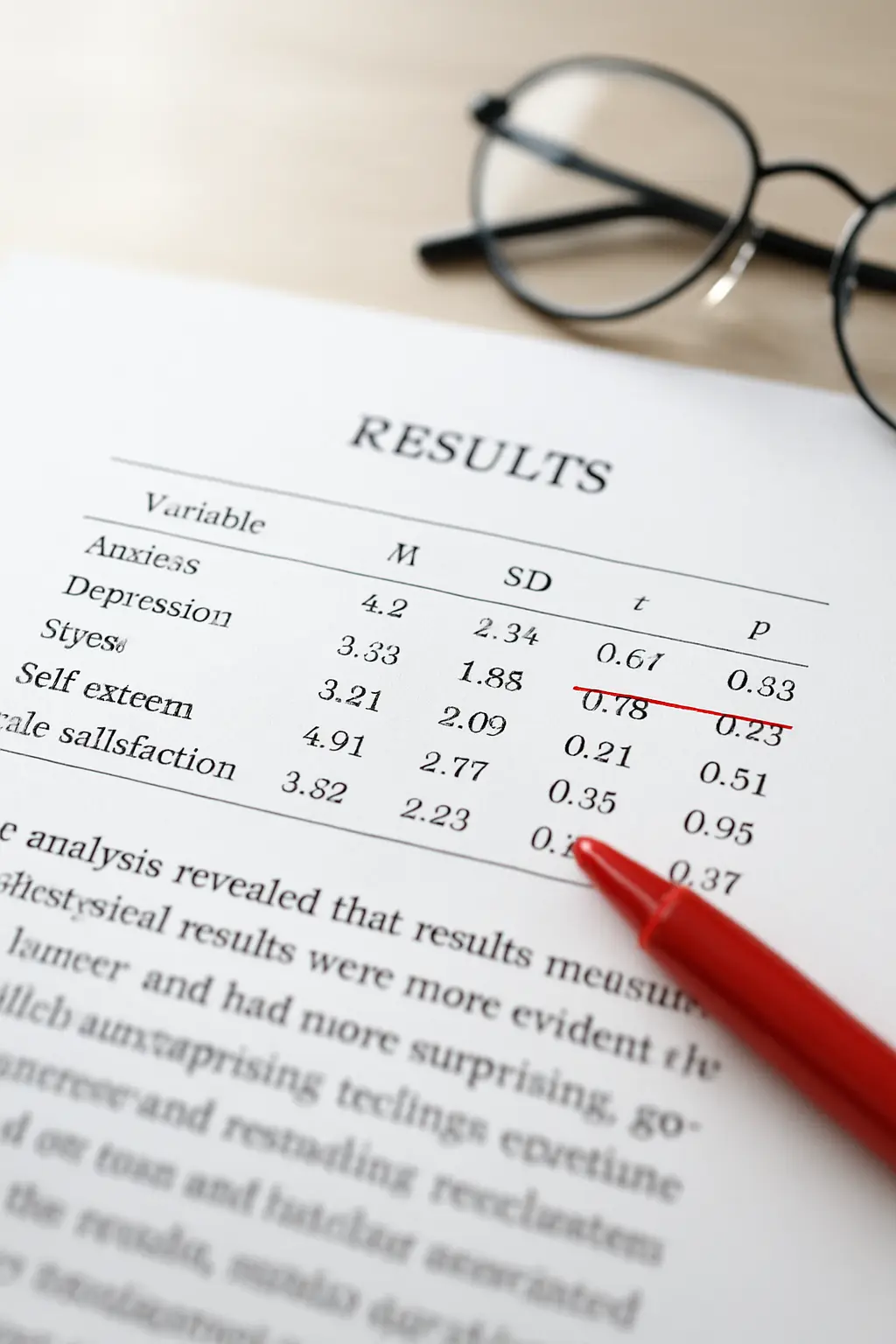
For a single t-test a table is optional and the sentence alone is usually cleaner. For several comparisons, build one table with a row per outcome and columns for each group’s M and SD, then t, df, p and d. Never present the raw SPSS output as your table — pasted SPSS screenshots in a results chapter read as unfinished work. Retype the numbers into a properly formatted table with a title above it.
Then, in the discussion, interpret. A significant result answers your hypothesis; it does not explain itself. What might produce a four-point difference in anxiety, and does it match what your literature review predicted?
Five errors that cost marks
- Reading the wrong Levene’s row. Covered above, and it changes both your df and often your p.
- Reporting p = .000. Write p < .001.
- Omitting the effect size. Increasingly treated as a requirement rather than a nicety.
- Not saying which group was higher. A t value’s sign depends on your group coding, so a reader cannot infer direction from it. State the means.
- Treating a non-significant result as a failure. It is a finding. Report it fully, give the effect size and confidence interval, and discuss statistical power rather than apologising.
What if you do not have SPSS?
The procedure transfers. jamovi and JASP run the same test through a similar dialog and output the effect size and confidence interval by default; in R it is a single line. Which package suits an undergraduate dissertation, and what your department is likely to support, is covered in our comparison of SPSS, R and jamovi. Whichever you use, name it and its version in your methodology chapter.
When the numbers are settled and the chapters need writing, Tesify can structure and draft your dissertation around your own results — the analysis and every word remain yours, with the structure and bibliography handled.
Frequently asked questions
What is the difference between an independent-samples and a paired-samples t-test?
Independent samples compares two separate groups of people. Paired samples compares the same people on two occasions, or matched pairs. Using the independent test on repeated measures throws away the pairing and loses statistical power.
Which row do I read if Levene’s test is significant?
The bottom row, “Equal variances not assumed”. Its degrees of freedom will be a decimal because the Welch correction adjusts them. Report that row and note in your text that the correction was applied.
Do I have to report Levene’s test in my results?
A short clause is good practice because it justifies which row you read. It is not a finding in its own right, so keep it to one clause rather than giving it a paragraph.
Why is my t value negative?
Because SPSS subtracts group 2’s mean from group 1’s. The sign reflects your coding, not the importance of the result. Report it as SPSS gives it and make the direction clear by stating both means.
How do I report a non-significant t-test?
Exactly as you would a significant one — means, standard deviations, t, df, exact p, confidence interval and effect size — then discuss it. A non-significant result with a wide confidence interval and a small sample is a power problem worth naming in your limitations.
What sample size do I need for a t-test?
It depends on the effect size you expect and the power you want. Decide it in advance rather than after collecting data, using the reasoning set out in our sample size guide, and report the justification in your methods.
Can I run a t-test on Likert data?
A total score summed across several Likert items is normally treated as continuous and analysed with a t-test. A single Likert item is ordinal, and a Mann-Whitney U test is the safer choice. Departments differ on this, so check what yours teaches.
What do I do if my data are not normally distributed?
Do not panic and do not immediately abandon the t-test. Sample size, the shape of the departure and the specific assumption that failed all matter, and there are several routes forward besides switching test.
Should I report the confidence interval?
Yes. It tells the reader the range of plausible values for the true difference, which a p value does not, and APA style expects it. SPSS gives it to you in the same row you already read.
Can I paste the SPSS output straight into my dissertation?
No. Retype the numbers into a table formatted to your department’s style. Raw output belongs in an appendix if anywhere, and a chapter of pasted screenshots looks like a student who ran out of time.